C Programming, Graphics, Linux, macOS, Programming, Simulation

Using wx_bgi_graphics With OpenLB

April 19, 2026 by Hammad Rauf

Read Time:16 Minute, 24 Second

Introduction

This article walks through a compact but surprisingly fun combo: running an OpenLB flow simulation while using wx_bgi_graphics to paint the results live in a window.

At a high level, the demo connects:

OpenLB: an open-source C++ framework for computational fluid dynamics based on the Lattice Boltzmann Method (LBM).
wx_bgi_graphics: a modern, cross-platform (Windows, Linux, macOS) BGI-style drawing API delivered as a shared library. It’s designed to make 2D (and simple 3D-style) rendering approachable from C/C++, Python and Free-Pascal (and potentially others, depending on bindings).

The emphasis here is on how the program uses wx_bgi_graphics to open a window, draw frames, and update visuals in a simulation loop. OpenLB concepts are introduced only to the extent needed to understand where the data comes from and how often the visualization updates.

Demo source (OpenLB + wx_bgi_graphics integration): https://github.com/Andromedabay/wx_bgi_graphics/tree/main/examples/cpp/openlb-demo
wx_bgi_graphics source: https://github.com/Andromedabay/wx_bgi_graphics
wx_bgi_graphics OpenLB-Support guide: https://github.com/Andromedabay/wx_bgi_graphics/blob/main/docs/user-guide/OpenLB-Support.md
OpenLB homepage: https://www.openlb.net/

What the demo is doing (big picture)

At runtime, the program keeps two gears turning: OpenLB
advances the physics, and wx_bgi_graphics turns those numbers into something
you can actually watch. Conceptually, it’s a tight loop:

Initialize the problem
setup: build the demo geometry using wx_bgi_graphics primitives (and
label/annotate it so it can be reused by external tooling such as OpenLB).
Initialize wx_bgi_graphics (open a window,
configure drawing state).
Time-step loop: advance the CFD solution
(collide-and-stream) and periodically extract scalar/vector quantities
(e.g., velocity magnitude, density, vorticity).
Render loop: map simulation values to pixels/colors
and draw primitives (points, lines, text, optional overlays) to form each
frame.
Handle input (keys/mouse) and exit cleanly.

OpenLB commonly outputs results for post-processing tools
(e.g., VTK/ParaView). This demo instead emphasizes an immediate-mode,
interactive window for learning, rapid iteration, and
“see-it-while-it-runs” feedback—exactly the niche where a simple BGI-style API
is convenient.

Prerequisites and build ingredients

C/C++ toolchain: a recent
GCC/Clang (recommended for this demo). wx_bgi_graphics itself supports
MSVC, but the author could not compile the latest OpenLB release with
MSVC—so this particular OpenLB demo is best treated as
Linux/WSL2/macOS-oriented (tested on Linux).
wxWidgets runtime/development files:
wx_bgi_graphics uses wxWidgets under the hood to create windows and draw.
wx_bgi_graphics shared library: built from
https://github.com/Andromedabay/wx_bgi_graphics and made discoverable at
runtime (e.g., via LD_LIBRARY_PATH on Linux/macOS or PATH on
Windows).
OpenLB: obtained from https://www.openlb.net/ (or
your preferred mirror). The demo’s build expects OpenLB headers and
libraries in a known location.

Platform note: wx_bgi_graphics is cross-platform, but
this specific OpenLB integration demo is primarily intended for Linux, WSL2, or
macOS due to the OpenLB/MSVC build limitation mentioned above.

Architecture overview: OpenLB compute + wx_bgi_graphics render

Geometry from drawing primitives (and why labeling matters)

In this workflow, wx_bgi_graphics isn’t only used to
visualize results—it can also be used to sketch the geometry itself
using familiar primitives (lines, rectangles, circles, polygons). Those shapes
can be labeled (e.g., “inlet”, “outlet”, “wall”, “obstacle”) so the same
geometry description can be interpreted consistently when you hand it off to
external software such as OpenLB for boundary assignment.

Inlet
label choose inflow boundary (velocity or pressure)
Outlet
label choose outflow / pressure reference boundary
Wall
label choose no-slip (bounce-back) boundary
Solid
obstacle label mark solid region inside the flow domain

The cleanest way to think about this program is as two
subsystems with a simple interface between them:

Simulation (OpenLB)	Visualization (wx_bgi_graphics)
Defines the lattice, physics, and boundary conditions; advances the solver in time steps.	Creates a window; draws primitives each frame; optionally handles input and overlays (HUD text, axes, legends).
Provides data fields (e.g., velocity magnitude at lattice nodes).	Maps data values to colors/positions and draws them (pixels/points/rectangles/lines).
Controls when to sample/output results (every N steps).	Controls refresh rate and any interpolation/downsampling used for display.

wx_bgi_graphics OpenLB-Support: what it adds

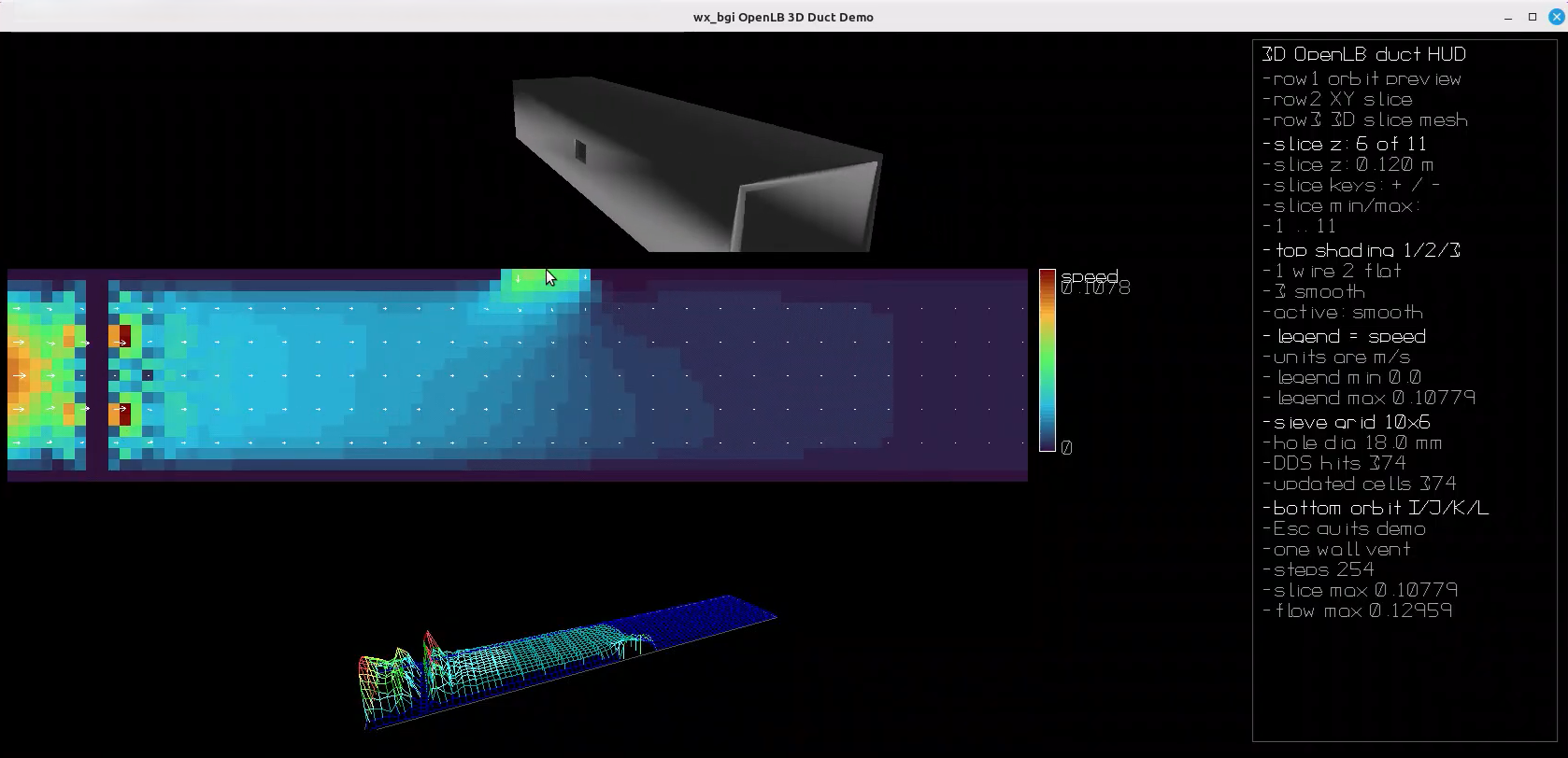
The demo doesn’t just “use wx_bgi_graphics for drawing.” It
leans on wx_bgi_graphics’ OpenLB-Support layer to make the end-to-end
workflow smooth: build a duct and sieve as labeled solids, materialize those
labels into the OpenLB geometry, then render both a 3D preview and live slice
diagnostics.

Geometry authoring via
primitives: draw the domain (walls/obstacles) using the same API
you’ll later use for visualization.
Labeling / tagging:
assign integer/material IDs (or named tags, depending on your workflow) to
pixels/regions so external code can interpret “what is what”.
Bridging helpers: small
utilities that turn those labels into something OpenLB can consume
(typically: material assignment and boundary selection).
Visualization helpers:
convenience routines/patterns to sample fields and render them efficiently
(e.g., scaling, palettes, overlays).

Walkthrough of the demo’s key functions

Instead of treating this as a generic “OpenLB + graphics”
integration, let’s follow the demo the way the code does. These four functions
are the backbone of the interactive experience:

main() boots everything:
window + cameras + DDS scenes, creates and validates the OpenLB geometry,
runs the step/render loop, and presents frames.
sampleLongitudinalSection()
samples a 2D slice from the 3D simulation and produces the scalar/vector
grids that the UI draws.
rebuildFlowPerspectiveScene()
rebuilds a 3D “height mesh” view of the slice using wx_bgi_graphics
world-space line primitives.
drawHud() draws the
right-hand info panel: controls, slice position, legend details, and
materialization stats.

main(): session setup, simulation loop, and rendering

The demo’s main() is essentially a story in three acts:

Parse flags (test mode +
shading mode) so the demo can run quickly in CI-like runs or with a
preferred render style.
Start wx_bgi_graphics + build
the DDS scene: the window is created with wxbgi_openlb_begin_session(),
and the 3D duct geometry is built via DDS solids (boxes +
union/difference) in buildDdsPipeScene().
Run the main step/render loop:
advance lattice.collideAndStream()
a few steps per frame, sample a slice for 2D overlays, rebuild the 3D
slice mesh scene, then draw everything (preview, 2D field grids, 3D mesh,
HUD) and present.

int main(int argc, char **argv)
{
    bool testMode = false;
    int solidMode = kModeSmooth;
    for (int i = 1; i < argc; ++i)
    {
        if (std::strcmp(argv[i], "--test") == 0)
            testMode = true;
        else if (std::strcmp(argv[i], "--wireframe") == 0)
            solidMode = kModeWireframe;
        else if (std::strcmp(argv[i], "--flat") == 0)
            solidMode = kModeFlat;
        else if (std::strcmp(argv[i], "--shaded") == 0 || std::strcmp(argv[i], "--smooth") == 0)
            solidMode = kModeSmooth;
    }

    wxbgi_openlb_begin_session(windowW, windowH, "wx_bgi OpenLB 3D Duct Demo");
    setbkcolor(BLACK);
    cleardevice();

    const SieveLayout sieveLayout = buildDdsPipeScene(converter);
    wxbgi_cam_create("pipe3d_preview", WXBGI_CAM_PERSPECTIVE);
    wxbgi_cam_set_scene("pipe3d_preview", "default");

    wxbgi_dds_scene_create("flow3d");
    wxbgi_cam_create("pipe3d_flow3d", WXBGI_CAM_PERSPECTIVE);
    wxbgi_cam_set_scene("pipe3d_flow3d", "flow3d");

    // ... OpenLB geometry + lattice setup omitted here for brevity ...

    while (wxbgi_openlb_pump())
    {
        for (int step = 0; step < stepsPerFrame; ++step, ++iT)
        {
            updateBoundaryValues(iT, converter, geometry, lattice);
            lattice.collideAndStream();
        }

        const float sliceValueMax = std::max(sampleLongitudinalSection(lattice,
                                                                       converter,
                                                                       geometry,
                                                                       sliceZ,
                                                                       sliceCols,
                                                                       sliceRows,
                                                                       scalar,
                                                                       vectors),
                                             1e-6f);
        const float sliceZPhys = static_cast<float>(converter.getPhysLength(sliceZ));
        rebuildFlowPerspectiveScene(converter, sliceCols, sliceRows, scalar, sliceValueMax, sliceZPhys);

        cleardevice();
        wxbgi_render_dds("pipe3d_preview");

        wxbgi_field_draw_scalar_grid(layout.fieldLeft, layout.fieldTop,
                                     sliceCols, sliceRows,
                                     scalar.data(), static_cast<int>(scalar.size()),
                                     kFieldCellPx,
                                     0.f, sliceValueMax,
                                     WXBGI_FIELD_PALETTE_TURBO);

        wxbgi_field_draw_vector_grid(layout.fieldLeft, layout.fieldTop,
                                     sliceCols, sliceRows,
                                     vectors.data(), static_cast<int>(vectors.size()),
                                     kFieldCellPx,
                                     12.f, 3, WHITE);

        wxbgi_render_dds("pipe3d_flow3d");
        drawHud(sliceZ, sliceZPhys, sliceIndexMin, sliceIndexMax,
                layout.hudLeft, layout.hudTop, layout.hudH,
                sliceValueMax, maxPhysVelocity, iT,
                materializeStats, solidMode, sieveLayout);

        if (!wxbgi_openlb_present())
            break;
    }

    return 0;
}

A few wx_bgi_graphics/OpenLB-support calls are doing a lot
of heavy lifting here:

wxbgi_openlb_begin_session(...)
creates the window and sets up an event/present loop that plays nicely
with the OpenLB stepping.
buildDdsPipeScene(converter) builds
the 3D duct/sieve geometry using wx_bgi_dds + wxbgi_solid primitives, and
tags objects with external attributes (for example, the sieve is tagged
with OpenLB role/material/boundary attributes).
wxbgi_render_dds(cameraName)
renders a DDS scene from the specified camera into the current frame
buffer.
wxbgi_field_draw_scalar_grid, wxbgi_field_draw_vector_grid,
and wxbgi_field_draw_scalar_legend
wxbgi_openlb_present() presents the
composed frame (and typically synchronizes with the windowing backend).

sampleLongitudinalSection(): turning a 3D lattice into 2D arrays

This function is the bridge between “simulation space” and
“UI space”. Given a Z index (sliceZ), it walks an X×Y plane, samples the OpenLB velocity, and
fills two buffers:

scalar[y*cols + x] stores the velocity
magnitude at each cell (used for the colored grid and legend).
vectors[(y*cols + x)*2 + 0/1]
stores (v_x, v_y) for a 2D vector overlay (used
for the arrow/grid vectors panel).
The return value is maxMagnitude, used
to normalize colors and heights consistently for that frame.

float sampleLongitudinalSection(SuperLattice<T, DESCRIPTOR> &lattice,
                                const UnitConverter<T, DESCRIPTOR> &converter,
                                const SuperGeometry<T, 3> &geometry,
                                int sliceZ,
                                int cols,
                                int rows,
                                std::vector<float> &scalar,
                                std::vector<float> &vectors)
{
    lattice.setProcessingContext(ProcessingContext::Evaluation);
    SuperLatticePhysVelocity3D<T, DESCRIPTOR> velocity(lattice, converter);

    float maxMagnitude = 0.f;
    for (int y = 0; y < rows; ++y)
    {
        for (int x = 0; x < cols; ++x)
        {
            const std::size_t scalarIdx = static_cast<std::size_t>(y * cols + x);
            const std::size_t vectorIdx = scalarIdx * 2;

            scalar[scalarIdx] = 0.f;
            vectors[vectorIdx + 0] = 0.f;
            vectors[vectorIdx + 1] = 0.f;

            const int material = geometry.get(0, x, y, sliceZ);
            if (material != kMatFluid && material != kMatInflow &&
                material != kMatOutflow &&
                material != kMatSideVent)
                continue;

            T output[3] = {};
            const int input[4] = {0, x, y, sliceZ};
            if (!velocity(output, input))
                continue;

            const float vx = static_cast<float>(output[0]);
            const float vy = static_cast<float>(output[1]);
            const float vz = static_cast<float>(output[2]);
            const float magnitude = std::sqrt(vx * vx + vy * vy + vz * vz);

            scalar[scalarIdx] = magnitude;
            vectors[vectorIdx + 0] = vx;
            vectors[vectorIdx + 1] = vy;
            maxMagnitude = std::max(maxMagnitude, magnitude);
        }
    }

    return maxMagnitude;
}

Notice the material check (geometry.get(...)) before sampling
velocity. This keeps the slice clean by ignoring walls/solids and only sampling
the materials that represent flow regions (fluid, inflow, outflow, side vent).

rebuildFlowPerspectiveScene(): building a 3D “slice mesh” with world lines

This function creates the third row’s 3D view. Instead of
drawing pixels, it rebuilds an entire DDS scene (named flow3d) every frame
using world-space line primitives:

Switch to the flow3d DDS scene
and activate the dedicated camera (pipe3d_flow3d).
Draw a rectangular outline on
the slice plane (the duct footprint).
Draw a grid of line strips in X
and Y where height encodes speed: each line endpoint gets a Z
offset proportional to scalar[idx] / maxMagnitude.
Add sparse vertical “spikes” as
an extra cue for magnitude.
Restore the default scene/camera
so the preview view continues to render normally.

void rebuildFlowPerspectiveScene(const UnitConverter<T, DESCRIPTOR> &converter,
                                 int cols,
                                 int rows,
                                 const std::vector<float> &scalar,
                                 float maxMagnitude,
                                 float sliceZPhys)
{
    const float dx = static_cast<float>(converter.getPhysDeltaX());
    const float baseZ = sliceZPhys;
    const float heightScale = 0.18f;

    wxbgi_dds_scene_set_active("flow3d");
    wxbgi_dds_scene_clear("flow3d");
    wxbgi_cam_set_active("pipe3d_flow3d");

    setcolor(DARKGRAY);
    wxbgi_world_line(0.f, 0.f, baseZ, static_cast<float>(kPipeLength), 0.f, baseZ);
    wxbgi_world_line(static_cast<float>(kPipeLength), 0.f, baseZ,
                     static_cast<float>(kPipeLength), static_cast<float>(kPipeWidth), baseZ);
    wxbgi_world_line(static_cast<float>(kPipeLength), static_cast<float>(kPipeWidth), baseZ,
                     0.f, static_cast<float>(kPipeWidth), baseZ);
    wxbgi_world_line(0.f, static_cast<float>(kPipeWidth), baseZ, 0.f, 0.f, baseZ);

    for (int y = 0; y < rows; ++y)
    {
        for (int x = 0; x < cols - 1; ++x)
        {
            const std::size_t idx0 = static_cast<std::size_t>(y * cols + x);
            const std::size_t idx1 = idx0 + 1;
            const float x0 = (static_cast<float>(x) + 0.5f) * dx;
            const float x1 = (static_cast<float>(x + 1) + 0.5f) * dx;
            const float yw = (static_cast<float>(y) + 0.5f) * dx;
            const float z0 = baseZ + (maxMagnitude > 1e-6f ? scalar[idx0] / maxMagnitude : 0.f) * heightScale;
            const float z1 = baseZ + (maxMagnitude > 1e-6f ? scalar[idx1] / maxMagnitude : 0.f) * heightScale;
            setcolor(paletteColorForScalar(0.5f * (scalar[idx0] + scalar[idx1]), maxMagnitude));
            wxbgi_world_line(x0, yw, z0, x1, yw, z1);
        }
    }

    // ... second pass draws Y-direction strips; third pass adds sparse vertical lines ...

    wxbgi_dds_scene_set_active("default");
    wxbgi_cam_set_active("pipe3d_preview");
}

In the real demo, the function continues with two more
loops: one draws the Y-direction strips (connecting (x, y) to (x, y+1)), and another
draws sparse vertical lines. The excerpt above is kept short, but every line
shown is copied directly from the demo.

drawHud(): the right-hand status panel

The HUD is a great example of why wx_bgi_graphics feels
productive: it’s just immediate-mode drawing. drawHud() draws a bordered panel and
then prints a series of bullet lines that make the demo self-explanatory while
it runs.

Navigation: tells you
which row is which, and the orbit controls (I/J/K/L) and slice controls
(+/-).
Slice position: shows
both the lattice index and the physical Z location in meters.
Render mode:
wireframe/flat/smooth selection, matching keys 1/2/3.
Legend: clarifies that
the color ramp represents speed in m/s, with the per-frame max.
OpenLB materialization stats:
matched
and updated
counters from WxbgiOpenLbMaterializeStats
show how the DDS geometry “hits” the lattice.

void drawHud(int sliceZ,
              float sliceZPhys,
              int sliceMin,
              int sliceMax,
              int hudLeft,
              int hudTop,
              int hudHeight,
              float maxMagnitude,
              float maxPhysVelocity,
              std::size_t steps,
               const WxbgiOpenLbMaterializeStats &materializeStats,
               int renderMode,
               const SieveLayout &sieveLayout)
{
    const int lineStep = 22;
    int lineY = hudTop;
    auto drawBullet = [&](const char *text, int color = LIGHTGRAY)
    {
        setcolor(color);
        outtextxy(hudLeft, lineY, const_cast<char *>("-"));
        outtextxy(hudLeft + 14, lineY, const_cast<char *>(text));
        lineY += lineStep;
    };

    setcolor(DARKGRAY);
    rectangle(hudLeft - 10, hudTop - 8, hudLeft + kHudPanelWidth - 4, hudTop + hudHeight - 8);
    setcolor(WHITE);
    outtextxy(hudLeft, lineY, const_cast<char *>("3D OpenLB duct HUD"));
    lineY += lineStep + 4;

    drawBullet("row1 orbit preview");
    drawBullet("row2 XY slice");
    drawBullet("row3 3D slice mesh");

    char line[160] = {};
    std::snprintf(line, sizeof(line), "slice z: %d of %d", sliceZ, sliceMax);
    drawBullet(line, WHITE);

    std::snprintf(line, sizeof(line), "active: %s", renderModeLabel(renderMode));
    drawBullet(line);

    std::snprintf(line, sizeof(line), "DDS hits %d", materializeStats.matched);
    drawBullet(line);

    std::snprintf(line, sizeof(line), "steps %zu", steps);
    drawBullet(line);

    std::snprintf(line, sizeof(line), "flow max %.5f", maxPhysVelocity);
    drawBullet(line);
}

The demo’s full drawHud() prints more detail (legend min/max,
sieve grid dimensions, hole diameter, and the key list). The snippet above is a
real excerpt, shortened to highlight the pattern: a reusable “bullet line”
helper + straightforward outtextxy()
calls.

Dictionary of key terms (OpenLB + LBM)

Term	Meaning (in this demo’s context)
Lattice (OpenLB)	The regular grid of cells (and associated particle distribution functions) where the Lattice Boltzmann Method is solved. Think of it as the simulation’s “computational canvas”: every cell holds state used to compute density and velocity.
Boundary conditions	Rules applied at the edges of the domain (and on obstacles) that enforce physical behavior such as inflow velocity, outflow pressure, or no-slip walls. In practice, this is where geometry labels like inlet/wall turn into solver constraints.
Collide-and-stream	The core LBM update step: “collision” relaxes distributions toward equilibrium locally; “streaming” propagates distributions to neighboring cells. Repeating this over many iterations advances the flow in time.
Parallelization (OpenLB)	OpenLB can distribute the lattice across multiple CPU cores (and across multiple nodes via MPI in many setups). Parallel performance depends on domain decomposition, communication overhead, and how much work happens per cell per step.
Mesh / lattice cell size	The spatial resolution of the simulation. Smaller cells (finer lattice) capture more detail but increase cost roughly with the number of cells. For live rendering, you may downsample the lattice when drawing so the simulation can remain responsive.

Running the demo quickly (Bash scripts)

The demo folder includes two helper scripts that are the
quickest way to get from zero to a running window. The Linux script is fully
automated (dependencies, cloning, CMake configure/build, and run), and it has
been tested.

run_openlb_pipe_3d_demo.sh (Linux / Debian / Ubuntu
/ WSL.2)
run_openlb_pipe_3d_demo_macos.sh (macOS)

Install dependencies (Linux
script): optionally installs required packages via apt (can be
skipped with --skip-system-packages).
Fetch sources: reuses an
existing checkout when possible, otherwise it can clone wx_bgi_graphics
(and clones the public OpenLB release to ${OPENLB_ROOT:-/tmp/openlb-release}).
Configure, build, run:
configures CMake with -DWXBGI_ENABLE_OPENLB=ON, builds the wxbgi_openlb_pipe_3d_demo
target, then runs it (interactive: --smooth, validation: --test).

# Linux / WSL2 (Debian/Ubuntu family)
./run_openlb_pipe_3d_demo.sh

# macOS
./run_openlb_pipe_3d_demo_macos.sh

# Optional quick validation run (Linux script)
./run_openlb_pipe_3d_demo.sh --test

Quick troubleshooting

“Library not found” on startup: confirm the loader
path (LD_LIBRARY_PATH / PATH) includes the wx_bgi_graphics shared library
directory.
Window opens but nothing changes: check whether the
simulation is rendering every N steps (render interval too large can look
frozen).
Low FPS: reduce the number of lattice cells drawn
per frame (downsample) or render less frequently.
Remote/headless machines: GUI rendering typically
needs an active display server (e.g., X11/Wayland on Linux).

Wrap-up

This demo is a handy template for pairing a heavyweight CFD engine (OpenLB) with a lightweight, approachable drawing API (wx_bgi_graphics). Once the “fields to pixels” bridge is in place, you can iterate fast: add new view modes, draw vectors or streamlines, drop in a color legend, and make the display interactive—without waiting for a full post-processing round-trip.

Categories

Andromedabay Store